Mastering Excel: The Ultimate Techniques for Labeling Your Cell Arrays

Quick Links

• How to Create a Name for a Cell or a Range of Cells Using the Name Box
• How to Edit Names Using the Name Manager
• How to Delete a Name Using the Name Manager
• How to Create a Name Using the “New Name” Dialog Box
• How to Use a Name to Represent a Constant Value

When creating formulas in Excel, you can reference cells from another part of the worksheet in your formulas. But if you have a lot of formulas, all those cell references can get confusing. There’s an easy way to remove the confusion.

Excel includes a feature, called “Names”, that can make your formulas more readable and less confusing. Instead of referencing a cell or range of cells, you can assign a name to that cell or range and use that name in formulas. This will make your formulas much easier to understand and maintain.

Related: How to Use VLOOKUP in Excel

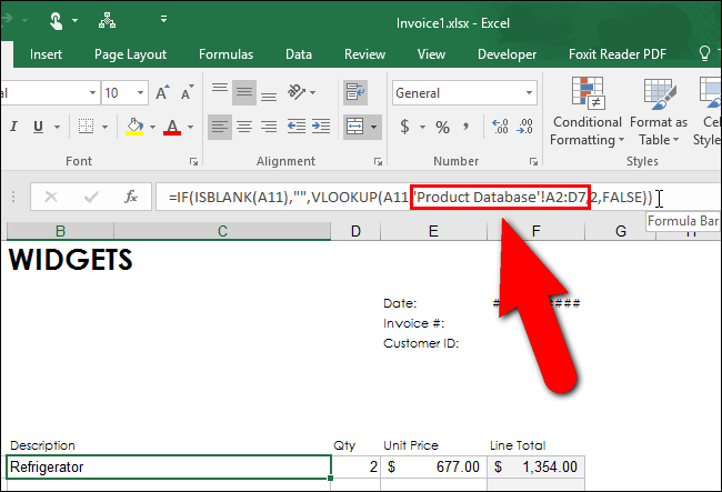
In the formula below, we reference a range of cells (in bold) from another worksheet, called “Product Database”, in the same workbook. In this case, the name of the worksheet gives us a good idea as to what’s contained in the range of cells, “A2:D7”. However, we could use a name for this range of cells to make the formula shorter and easier to read.

=IF(ISBLANK(A11),””,VLOOKUP(ALL,’Product Database’!A2:D7,2,FALSE))

NOTE: For more information about the VLOOKUP function used in the formula above, see our article about using VLOOKUP in Excel . You can also learn how to use the “IF” function and other useful functions .

How to Create a Name for a Cell or a Range of Cells Using the Name Box

To assign a name to a range of cells, select the cells you want to name. The cells don’t have to be contiguous. To select non-contiguous cells, use the “Ctrl” key when selecting them.

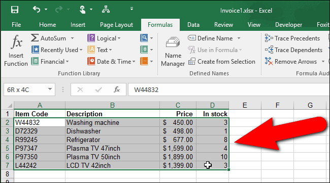
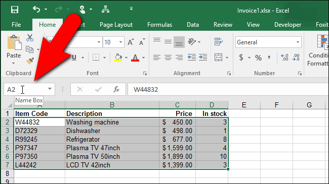
Click the mouse in the “Name Box” above the cell grid.

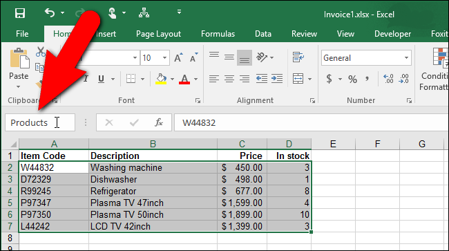
Type a name for the range of cells in the box and press “Enter”. For example, we called the selected cells on our “Product Database” worksheet “Products”. There are syntax rules you must abide by when choosing a name. You can only begin a name with a letter, an underscore (_), or a backslash (\). The rest of the name can consist of letters, numbers, periods, and underscores. There are additional syntax rules about what’s valid and not when defining names.

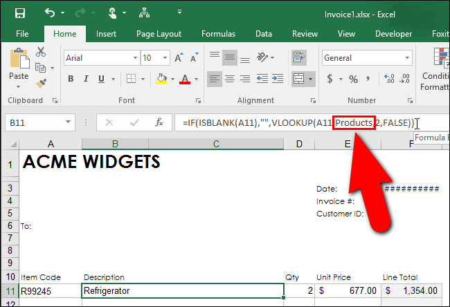
Remember the formula from the beginning of this article? It contained a reference to the “Products Database” worksheet in the workbook and a range of cells on the that worksheet. Now, that we created the “Products” name to represent the range of cells on our “Products Database” worksheet, we can use that name in the formula, shown in bold below.

=IF(ISBLANK(A11),””,VLOOKUP(ALL,Products,2,FALSE))

NOTE: When creating a name using the “Name Box”, the scope of the name defaults to the workbook. That means that the name is available to be used on any worksheet in the current workbook without referencing a specific worksheet. You can choose to limit the scope to a specific worksheet so the worksheet name has to be used when referring to the name, such as in the example at the beginning of this article.

How to Edit Names Using the Name Manager

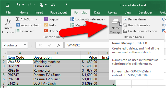
Excel provides a tool, called “Name Manager”, that makes it easy to find, edit, and delete the names in your workbook. You can also use the Name Manager to create names, if you want to specify more details about the name. To access the Name Manager, click the “Formulas” tab.

In the “Defined Names” section of the “Formulas” tab, click “Name Manager”.

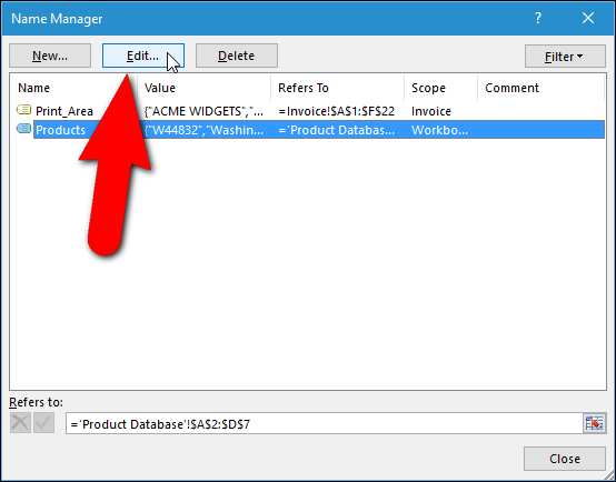
The Name Manager dialog box displays. To edit an existing name, select the name in the list and click “Edit”. For example, we’re going to edit the “Products” name.

The “Edit Name” dialog box displays. You can change the “Name” itself as well as add a “Comment” to the name, providing more details about what the name represents. You can also change the range of cells to which this name is assigned by clicking the “Expand Dialog” button on the right side of the “Refers to” edit box.

NOTE: You’ll see that the “Scope” drop-down list is grayed out. When you edit an existing name, you cannot change the “Scope” of that name. You must choose the scope when you first create the name. If you want the scope to be a specific worksheet, rather than the entire workbook, you can create a name in a way that allows you to specify the scope initially. We’ll show you how to do that in a later section.

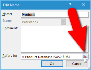
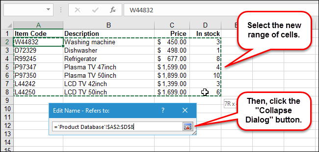
As an example, say we added another product to our “Product Database” and we want to include it in the cell range named “Products”. When we click on the “Expand Dialog” button, the “Edit Name” dialog box shrinks down to contain only the “Refers to” edit box. We select the range of cells directly on the “Product Database” worksheet, including the row containing the newly added product. The worksheet name and cell range are automatically entered into the “Refers to” edit box. To accept your selection and return to the full “Edit Name” dialog box, click the “Collapse Dialog” button. Click “OK” on the “Edit Name dialog box to accept the changes to the name.

WPS Office Premium ( File Recovery, Photo Scanning, Convert PDF)–Yearly

How to Delete a Name Using the Name Manager

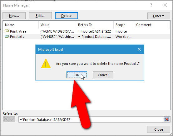
If you decide you don’t need a name anymore, it’s easy to delete it. Simply, access the “Name Manager” dialog box as we discussed in the previous section. Then, select the name you want to delete in the list of names and click “Delete”.

On the confirmation dialog box that displays, click “OK” if you’re sure you want to delete the selected name. You are returned to the “Name Manager” dialog box. Click “Close” to close it.

Epubor Ultimate for Mac:Helps you read books anywhere, including the best eBook Converter + eBook DRM Removal functions.

How to Create a Name Using the “New Name” Dialog Box

When you create a new name by selecting one or more cells and then entering a name in the “Name Box”, the default scope of the name is the entire workbook. So, what do you do if you want to limit the scope of a name to just a specific worksheet?

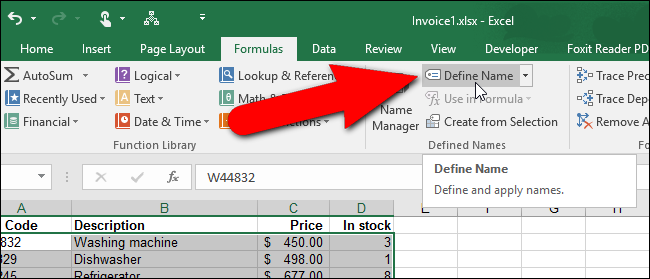
Select the cells to which you want to assign the name. Click the “Formulas” tab and then click “Define Name” in the “Defined Names” section.

NOTE: You don’t have to select the cells first. You can also select them using the “Expand Dialog” button later on, if you want.

DEX 3 RE is Easy-To-Use DJ Mixing Software for MAC and Windows Designed for Today’s Versatile DJ.

DEX 3 RE is everything you need without the clutter - the perfect 2-deck mixing software solution for mobile DJs or hard-core hobbiests. 
PCDJ DEX 3 RE (DJ Software for Win & MAC - Product Activation For 3 Machines)

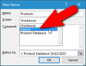
The “New Name” dialog box displays. Notice that it’s very similar to the “Edit Name” dialog box mentioned earlier. The main difference is that now you can change the scope of the name. Say we want to limit the scope of the name to just the “Invoice” worksheet. We would do this if we wanted to be able to use the same name for a range of cells on another worksheet.

First, we’ll enter the name we want to use, which in our case is “Products”. Remember the syntax rules when creating your name. Then, to limit the scope of the “Products” name to only the “Invoice” worksheet, we select that from the “Scope” drop-down list.

NOTE: The “New Name” dialog box can also be accessed by clicking “New” on the “Name Manager” dialog box.

Enter more details about the name, if desired, in the “Comment” box. If you didn’t select the cells to which you’re assigning the name, click the “Expand Dialog” button to the right of the “Refers to” edit box to select the cells the same way we did when we edited the name earlier. Click “OK” to finish creating the new name.

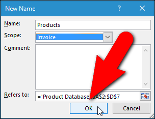
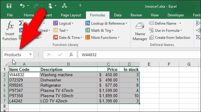
The name is automatically inserted into the same “Name Box” we used to assign a name to a range of cells at the beginning of this article. Now, we can replace the cell range reference (‘Product Database’!$A$2:$D:7) with the name (Products) in the formulas on the “Invoice” worksheet, like we did earlier in this article.

How to Use a Name to Represent a Constant Value

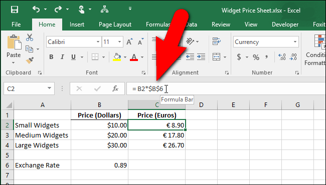
You don’t have to refer to cells when creating a name. You can use a name to represent a constant, or even a formula. For example, the worksheet below shows the exchange rate used to calculate the price in Euros for the various sizes of widgets. Because the exchange rate changes often, it would be useful if it was located in a place that’s easy to find and update. Since names are easy to edit, as discussed earlier, we can create a name to represent the exchange rate and assign a value to the name.

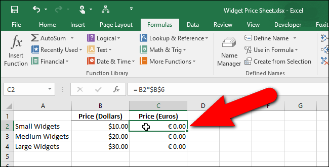
Notice the formula contains an absolute cell reference to a cell containing the current exchange rate. We’d rather use a name that will refer to the current exchange rate so it’s easier to change and formulas using the exchange rate are easier to understand.

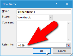
To create a name that will be assigned to a constant value, open the “New Name” dialog box by clicking the “Formulas” tab and then clicking “Define Name” in the “Defined Names” section. Enter a name to represent the constant value, such as “ExchangeRate”. To assign a value to this name, enter an equal sign (=) in the “Refers to” edit box followed by the value. There should not be a space between the equal sign and the value. Click “OK” to finish creating the name.

NOTE: If there’s a formula you use in many places in your workbook, you can enter that formula into the “Refers to” edit box so you can simply enter the name in every cell where you need to use the formula.

Now, we can use the new name in formulas where we want to use the exchange rate. When we click on a cell with a formula that contains an absolute cell reference , notice the result is “0.00”. That’s because we removed the exchange rate from the cell being referenced. We’ll replace that cell reference with the new name we created.

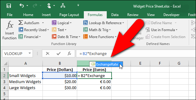
Highlight the cell reference (or other part of the formula you want to replace with a name) and start typing the name you created. As you type, any matching names display in a popup box. Select the name you want to insert into the formula by clicking on it in the popup box.

Jet Profiler for MySQL, Enterprise Version： Jet Profiler for MySQL is real-time query performance and diagnostics tool for the MySQL database server. Its detailed query information, graphical interface and ease of use makes this a great tool for finding performance bottlenecks in your MySQL databases.

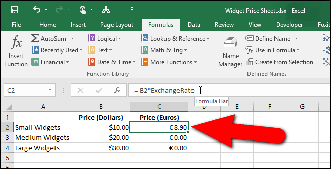
The name is inserted into the formula. Press “Enter” to accept the change and update the cell.

Note that the result is updated using the exchange rate referred to by the name.

Names are very useful if you create complex Excel workbooks with a lot of formulas. When you need to distribute your workbooks to others, using names makes it easier for others, as well as yourself, to understand your formulas.