Mastering Nested Selectors: Building Related Dropdown Menus in Excel

Quick Links

• Getting Started
• Adding and Naming Dependent Drop-Down List Items
• Creating the Dependent Drop-Down List

Does using a drop-down list in Microsoft Excel make data entry easier for you or your co-workers? If you said yes and want to go a step further, you can create a dependent drop-down list just as easily.

With a dependent drop-down list, you select the item that you want in the first list, and that determines the items that display as choices in the second one. For example, you might select a product, like a shirt, and then pick a size, a food item, like ice cream, and then pick a flavor, or an album, and then pick a song.

Getting Started

Obviously, you’ll need your first drop-down list set up and ready to go before you can create the dependent list. We have a complete tutorial with all of the details you need to create a drop-down list in Excel for a refresher, so be sure to check that out.

Related: How to Add a Drop-Down List to a Cell in Excel

Since setting up the second list follows the same basic process, we’ll start there. Then, we’ll move on to the dependency setup.

Glarysoft File Recovery Pro - Helps to recover your lost file/data, even permanently deleted data.

Adding and Naming Dependent Drop-Down List Items

For this tutorial, we’ll use departments in our company for the first drop-down list, and then employees in each department for the second list.

Our departments include Marketing, Finance, and Human Resources (HR), and each has three employees. These employees are who we need to add and name.

List the items for the dependent list, and then select the cells. This places the cells in a group so that you can name the group. With the cells selected, go up to the Name Box on the left side of the Formula Bar and enter a name for the cell group .

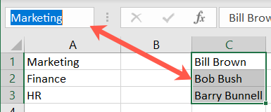
The names for each group should match the list items in your first dropdown.

Using our example, we’ll name our groups with the departments in our first list: Marketing, Finance, and HR.

Any DRM Removal for Win：Remove DRM from Adobe, Kindle, Sony eReader, Kobo, etc, read your ebooks anywhere.

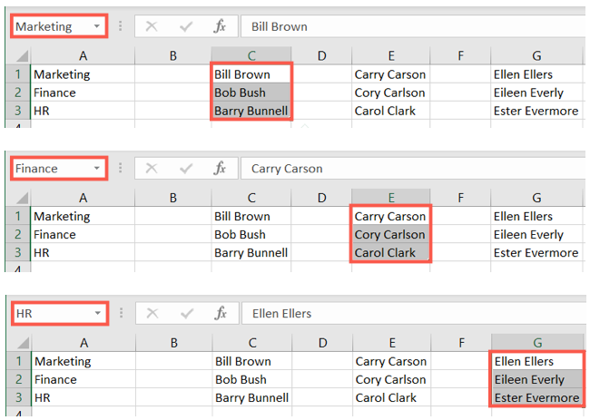
You can add the items for your dependent list on the same sheet where the list will reside or on a different one. For the purposes of this how-to, you’ll notice that we have everything on the same sheet.

Creating the Dependent Drop-Down List

Once all of your list items are in a sheet and named, it’s time to create the second drop-down list. You’ll use the Data Validation feature in Excel , just like when creating your first list.

Select the cell where you want the list. Then, go to the Data tab and click “Data Validation” in the Data Tools section of the ribbon.

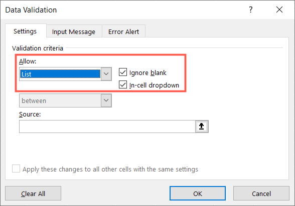
Choose the Settings tab in the pop-up window. Under Allow, pick “List,” and to the right, check the box for In-Cell Dropdown. Optionally, you can check the box to Ignore Blank cells if you like.

In the Source box, enter the formula below. Be sure to replace the cell reference in parentheses with the cell containing your first drop-down list.

=INDIRECT($B$6)

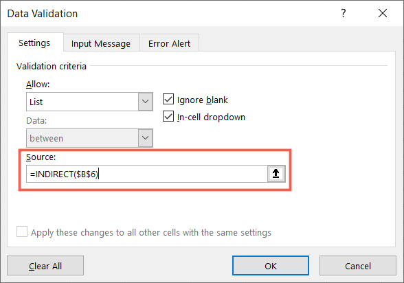
The INDIRECT function “returns the reference specified by a text string.” For additional details on this function, check out the Microsoft Support page.

If you’d like to include an Input Message or Error Alert, select those tabs in the pop-up window and enter the details. When you finish, click “OK” to add the drop-down list to the cell.

Now, give your list a test. When you select an item in the first drop-down list, you should see the items pertaining to your selection as options in the second list.

Jet Profiler for MySQL, Enterprise Version： Jet Profiler for MySQL is real-time query performance and diagnostics tool for the MySQL database server. Its detailed query information, graphical interface and ease of use makes this a great tool for finding performance bottlenecks in your MySQL databases.

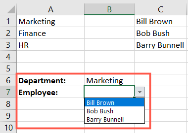
For quicker data entry for yourself or your collaborators, try a dependent drop-down list in Excel!